dhlabR

The National Biblioteket has million of digitised resources (books, manuscripts, newspapers, letters, etc.). As well as hosting an online norsk n-gram for quering the corpus, the DH-LAB is also creating its own tools for accessing and analysing their collections, including dhlabR an R package to directly interact with the corpus. It is still in development but some features work and allows accessing its massive corpus: you can have a look on their collections

National Biblioteket digital collection.

The package dhlabR interacts with the API of National Biblioteket. Although it does not allow to download full texts, you can query the collection, get the necessary metadata (including text IDs) and extracting text-derived outputs such as token frequencies or the text around keywords.

Using this package usually entail two steps:

Retrieve corpus metadata based on quering the corpus using given parameters such as author, title, year, language, type of document (e.g. book, newspaper, etc.), among others. This query is sent to the DH-LAB API and returns a table of matching documents, including document ID and associated metadata.
Request derived text data: term frequencies, concordances, collocations, etc. Instead of extracting full texts directly, you obtain representations (term frequencies, terms around keywords, etc.) tied to those document IDs, usually as a data frame or list that you can use in R for analysis and visualisation.

Here I provide a basic overview of some of these functions.

First, you need to install the package. Given that it is a beta version, it is not available via the usual channel but with the following (make sure to also install devtools if you haven’t used this package before).

Show code

# install.packages("devtools")
devtools::install_github("NationalLibraryOfNorway/dhlabR")

library(dhlabR)
library(tidyverse)

Once the package is loaded, you get access to different functions.

Retrieving the corpus metadata

get_document_corpus() queries the corpus available at NB and retrieve the associated metadata. This query is defined by particular parameters such as author, title, year, language, type of document (e.g. book, newspaper, journal, letter, etc.), among others. The following, for instance, extracts the metadata associated to texts stored as “digibok”, written by “Ibsen” between the years “1880” and “1890” (the argument to_year retrieves up to the define year, without including it). The argument limit sets the maximum number of items that can be retrieved. Here we are getting 37 rows, so setting it to “50” is fitting, so you do not miss any (careful because the default value is 10). This function returns a data frame, so I use glimpse() to have a sense of how the data looks like (you can also just type the name of the object).

Show code

# Get corpus
corpus <- get_document_corpus(
  doctype = "digibok", author = "Ibsen", 
  from_year = 1880, to_year = 1891,
  limit = 50)
corpus |> glimpse()

Rows: 43
Columns: 19
$ dhlabid       <named list> 100622339, 100619301, 100614233, 100329338, 10057…
$ urn           <named list> "URN:NBN:no-nb_digibok_2013073124012", "URN:NBN:n…
$ title         <named list> "Rosmersholm : skuespil i fire akter", "Nora ( Et…
$ authors       <named list> "Ibsen , Henrik", "Ibsen , Henrik", "Ibsen , Henr…
$ oaiid         <named list> "oai:nb.bibsys.no:998221073094702202", "oai:nb.bi…
$ sesamid       <named list> "48dfd8aca000073ca41028cb335f1ef4", "db3946047669…
$ isbn10        <named list> "", "", "", "", "", "", "", "", "", "", "", "", "…
$ city          <named list> "København", "Helsingissä", "København", "Københa…
$ timestamp     <named list> 18860101, 18800101, 18830101, 18830101, 18800101,…
$ year          <named list> 1886, 1880, 1883, 1883, 1880, 1886, 1880, 1881, 1…
$ publisher     <named list> "Gyldendalske Boghandels Forl.", "K.E. Holmin", "…
$ langs         <named list> "nob", "fin / nob", "nob", "nob", "fin / nob", "n…
$ subjects      <named list> "", "", "skjønnlitteratur/voksen", "", "", "", ""…
$ ddc           <named list> "", "", "", "", "", "", "", "", "", "", "", "", "…
$ genres        <named list> "drama", "", "", "fiction", "", "", "", "drama", …
$ literaryform  <named list> "Skjønnlitteratur", "Uklassifisert", "Uklassifise…
$ doctype       <named list> "digibok", "digibok", "digibok", "digibok", "digi…
$ ocr_creator   <named list> "dhlab", "dhlab", "dhlab", "nb", "nb", "dhlab", "…
$ ocr_timestamp <named list> 20221201, 20221201, 20221201, 20060101, 20060101,…

Notice that, instead of as characters or numerical values, the columns are formated as list-columns. This is because the API returns nested JSON, which the package converts into lists inside a tibble. Retrieving these values requires converting them. You can, for instance, transform them using map_chr() or map_int() depending on whether the underlying values are strings or numerical.¹

¹ If the list contains more than one value for each row (locations or publishers, for instance), you can use unnest(). You can use lengths() to check if that is the case.

Show code

corpus <- corpus |>
  mutate(title = map_chr(title, 1),
         dhlabid = map_int(dhlabid, 1))
corpus |> glimpse()

Rows: 43
Columns: 19
$ dhlabid       <int> 100622339, 100619301, 100614233, 100329338, 100571492, 1…
$ urn           <named list> "URN:NBN:no-nb_digibok_2013073124012", "URN:NBN:n…
$ title         <chr> "Rosmersholm : skuespil i fire akter", "Nora ( Et dukkeh…
$ authors       <named list> "Ibsen , Henrik", "Ibsen , Henrik", "Ibsen , Henr…
$ oaiid         <named list> "oai:nb.bibsys.no:998221073094702202", "oai:nb.bi…
$ sesamid       <named list> "48dfd8aca000073ca41028cb335f1ef4", "db3946047669…
$ isbn10        <named list> "", "", "", "", "", "", "", "", "", "", "", "", "…
$ city          <named list> "København", "Helsingissä", "København", "Københa…
$ timestamp     <named list> 18860101, 18800101, 18830101, 18830101, 18800101,…
$ year          <named list> 1886, 1880, 1883, 1883, 1880, 1886, 1880, 1881, 1…
$ publisher     <named list> "Gyldendalske Boghandels Forl.", "K.E. Holmin", "…
$ langs         <named list> "nob", "fin / nob", "nob", "nob", "fin / nob", "n…
$ subjects      <named list> "", "", "skjønnlitteratur/voksen", "", "", "", ""…
$ ddc           <named list> "", "", "", "", "", "", "", "", "", "", "", "", "…
$ genres        <named list> "drama", "", "", "fiction", "", "", "", "drama", …
$ literaryform  <named list> "Skjønnlitteratur", "Uklassifisert", "Uklassifise…
$ doctype       <named list> "digibok", "digibok", "digibok", "digibok", "digi…
$ ocr_creator   <named list> "dhlab", "dhlab", "dhlab", "nb", "nb", "dhlab", "…
$ ocr_timestamp <named list> 20221201, 20221201, 20221201, 20060101, 20060101,…

You can use the metadata, the information associated with each document, to better define your corpus of interest or your subsequent analysis.

Show code

corpus |>
  mutate(genres = map_chr(genres, 1)) |>
  count(genres)

          genres  n
1                24
2          drama 12
3        fiction  6
4 poetry / tekst  1

The example above retrieves a corpus of books (“digbok”: novels, monographs, plays, etc.), but defining the argument doctype differently allows accessing other materials, such as newspapers (“digavis”), journals and periodicals (“digitidsskrift”), letters and manuscripts (“digimanus”) or images (“digifoto”). The example below retrieves 10 newspapers published in 1905. Note that I am setting lang = NULL to avoid the defaul language (“nob”; bokmål, the official Norwegian language), which may make less sense in historical documents. The metadata contains potentially interesting information such as “title”, place of publication (“city”) or date of publication (“year” or “timestamp”).

Show code

newspapers <- get_document_corpus(
  doctype = "digavis", 
  from_year = 1905, to_year = 1906,
  lang = NULL,
  limit = 10)
newspapers |> glimpse()

Rows: 10
Columns: 19
$ dhlabid       <named list> 202158453, 200642308, 201285137, 203732055, 20315…
$ urn           <named list> "URN:NBN:no-nb_digavis_egersundsposten_null_null_…
$ title         <named list> "egersundsposten", "gjengangeren", "norskkundgjoe…
$ authors       <named list> "", "", "", "", "", "", "", "", "", ""
$ oaiid         <named list> "", "", "", "", "", "", "", "", "", ""
$ sesamid       <named list> "", "", "", "", "", "", "", "", "", ""
$ isbn10        <named list> "", "", "", "", "", "", "", "", "", ""
$ city          <named list> "Eigersund", "Horten", "Oslo", "", "Levanger", "S…
$ timestamp     <named list> 19050419, 19050902, 19051118, 19051129, 19051211,…
$ year          <named list> 1905, 1905, 1905, 1905, 1905, 1905, 1905, 1905, 1…
$ publisher     <named list> "", "", "", "", "", "", "", "", "", ""
$ langs         <named list> "", "", "", "", "", "", "", "", "", ""
$ subjects      <named list> "", "", "", "", "", "", "", "", "", ""
$ ddc           <named list> "", "", "", "", "", "", "", "", "", ""
$ genres        <named list> "", "", "", "", "", "", "", "", "", ""
$ literaryform  <named list> "", "", "", "", "", "", "", "", "", ""
$ doctype       <named list> "digavis", "digavis", "digavis", "digavis", "diga…
$ ocr_creator   <named list> "nb", "nb", "nb", "nb", "nb", "nb", "nb", "nb", "…
$ ocr_timestamp <named list> 20060101, 20060101, 20060101, 20060101, 20060101,…

Term frequencies per document

The function get_document_frequencies() search within the respective NB collections and computes ngram counts of the documents that are specified, an information that is contained in the corpus metadata retrieved in the previous step. The results can be plotted using regular R functions.

Let’s start from afresh and define the corpus we want to explore. Imagine that we want to track the relative importance of the terms “dame” and “kvinne” to refer to women during the first half of the 20^th century. We will focus on books, the literary realm. We first extract the metadata behind the digitised collection. As mentioned earlier, it is important to define a limit that is larger than the collection itself, so we don’t miss any text (this is basically done by trial and error). The resulting dataframe, containing information on 58,222 documents, is stored as an object named books.

Show code

books <- get_document_corpus(
  doctype = "digibok", 
  from_year = 1900, to_year = 1951,
  lang = NULL,
  limit = 100000) 
# |> distinct(dhlabid, .keep_all = TRUE)

We now use get_document_frequencies() to retrieve word counts of the terms we are interested in. The computation itself takes place in the NB server and we get the results. What this function is doing is to search for a list of particular words in the documents from the corpus we are studying, identified by their pids, which are stored in the object corpus and field urn. The function distinguish between lower- and upper-case letter, so make sure to expand the number of keywords accordingly if you think that finding upper-case characters is important. For comparison, it is important to include a term that is common enough to appear in all documents (e.g. “og” or “er”). Otherwise, you get only information on the documents providing hits.

Show code

wom_freq <- get_document_frequencies(
  pids = books$urn,
  words = c("dame", "damer", "kvinne", "kvinner", "og", "er"))
glimpse(wom_freq)

Rows: 163,909
Columns: 4
$ V1 <list> 100502131, 100502266, 100502268, 100502461, 100502533, 100502678, …
$ V2 <list> "dame", "dame", "dame", "dame", "dame", "dame", "dame", "dame", "d…
$ V3 <list> 2, 1, 1, 1, 1, 3, 19, 1, 1, 2, 1, 15, 1, 9, 3, 3, 9, 8, 15, 22, 3,…
$ V4 <list> 138288, 109973, 130050, 45193, 23226, 118260, 85964, 53291, 51249,…

The command above returns a data frame with 163909 rows. Notice that the API returns four unnamed columns referring to the document identifier, the term(s) we were looking for, the frequency those terms appear in that particular document and the total word count in that document. Also, as before, these fields are structured as lists. It is therefore a good idea to tidy this data frame up.

Show code

wom_freq <- wom_freq |>
  rename(dhlabid = V1,
         word = V2,
         count = V3,
         doc_length = V4) |>
  as_tibble() |>
  mutate(dhlabid = map_int(dhlabid, 1),
         word = map_chr(word, 1),
         count = map_int(count, 1),
         doc_length = map_int(doc_length, 1))
wom_freq

# A tibble: 163,909 × 4
     dhlabid word  count doc_length
       <int> <chr> <int>      <int>
 1 100502131 dame      2     138288
 2 100502266 dame      1     109973
 3 100502268 dame      1     130050
 4 100502461 dame      1      45193
 5 100502533 dame      1      23226
 6 100502678 dame      3     118260
 7 100503009 dame     19      85964
 8 100503166 dame      1      53291
 9 100503169 dame      1      51249
10 100503282 dame      2     174321
# ℹ 163,899 more rows

The resulting object now contains the information we were looking for and structured in a familiar way. Note that this object only contains the counts themselves. However, we have the document ids (dhlabid), so we could retrieve the metadata that was stored in the first object we retrieve (stored as books here), so we can make use of features such as “year” and “city” of publication, “author,”genres”, etc.² We therefore prepare merge both objects together, the one with the metadata and the one with the term frequencies.

² There are more fields but here we just focus on some of them.

It is important to realise that the data frame above is unbalanced because each row refers to a document where the particular term is mentioned at least once (but if it is not mentioned, there is no row). Counting the number of rows for each term makes this very clear. Recall that our corpus has 55,764 documents. The table below indicates the number of documents in which those terms are mentioned. The terms “er” and “og” show up in almost all of them (50,949 and 50,403, respectively) and we can perhaps safely argue that if those terms do not show up the document itself is probably unimportant or not very representative, so not having info on them (e.g. doc_lenght) is not going to affect our results.

Show code

wom_freq |>
  count(word)

# A tibble: 6 × 2
  word        n
  <chr>   <int>
1 dame    14953
2 damer   12373
3 er      53327
4 kvinne  14922
5 kvinner 15553
6 og      52781

In fact, however, the problem is less severe because there are documents which do not mention “og” but “er” (or the other terms) and vice versa, so the total number of documents is slightly higher (51,473; but not the full universe we started with). A potential solution is going back and add more terms to the search but we may not succeed in hitting all documents because a few of them might be very small documents anyway.

Show code

wom_freq |>
  count(dhlabid)

# A tibble: 53,877 × 2
     dhlabid     n
       <int> <int>
 1 100000002     4
 2 100000009     2
 3 100000011     3
 4 100000016     4
 5 100000017     3
 6 100000019     6
 7 100000022     2
 8 100000472     1
 9 100000473     2
10 100000474     2
# ℹ 53,867 more rows

More important is the unbalanced nature of the data frame above. Take into account, for instance, that if our search has found 3 instances of “og” in 1 document but none of the other terms, the data frame only contains one row for that document: the one indicating that word “og” has a count of 3 (and doc_lenght of “whatever”). We want though that the data frame contained 6 rows for each document, one for each word we are looking for, indicating a count of 0 when that is the case. The way to deal with is to use complete(), a commands that adds the rows with the categories that are missing (in our case, the terms that are not mentioned in the documents. The function complete() requires indicating the identifying field and the full set of categories present in the other field.

Show code

wom_freq <- wom_freq |>
  complete(dhlabid, 
           word = c("dame", "damer", "kvinne", "kvinner", "og", "er"))
wom_freq

# A tibble: 323,262 × 4
     dhlabid word    count doc_length
       <int> <chr>   <int>      <int>
 1 100000002 dame       10      42104
 2 100000002 damer       1      42104
 3 100000002 er        447      42104
 4 100000002 kvinne     NA         NA
 5 100000002 kvinner    NA         NA
 6 100000002 og       1349      42104
 7 100000009 dame       NA         NA
 8 100000009 damer      NA         NA
 9 100000009 er        534      61896
10 100000009 kvinne     NA         NA
# ℹ 323,252 more rows

The result is a data frame with 308,838 rows, which is the number of individual documents with at least 1 hit (51,473) times 6, the number of terms we searched for). We just need to fill in the gaps (NAs) with the adequate information, so we know not only the positive hits but also those with no hits (and the associated doc_lenght).

Show code

wom_freq <- wom_freq |>
  mutate(count = if_else(is.na(count), 0, count)) |>
  group_by(dhlabid) |>
  mutate(doc_length = mean(doc_length, na.rm = TRUE)) |>
  ungroup()
wom_freq

# A tibble: 323,262 × 4
     dhlabid word    count doc_length
       <int> <chr>   <dbl>      <dbl>
 1 100000002 dame       10      42104
 2 100000002 damer       1      42104
 3 100000002 er        447      42104
 4 100000002 kvinne      0      42104
 5 100000002 kvinner     0      42104
 6 100000002 og       1349      42104
 7 100000009 dame        0      61896
 8 100000009 damer       0      61896
 9 100000009 er        534      61896
10 100000009 kvinne      0      61896
# ℹ 323,252 more rows

Let’s then merge both objects. The original one also needs a bit of tuning. For simplicity, we just keep 4 fields of all the available metadata.

Show code

books_freq <- books |>
  as_tibble() |>
  select(dhlabid, year, city, authors, genres) |>
  mutate(dhlabid = map_int(dhlabid, 1),
         year = map_int(year, 1),
         city = map_chr(city, 1),
         authors = map_chr(authors, 1),
         genres = map_chr(genres, 1)) |>
  full_join(wom_freq, by = "dhlabid")
books_freq

# A tibble: 327,623 × 8
     dhlabid  year city   authors      genres word    count doc_length
       <int> <int> <chr>  <chr>        <chr>  <chr>   <dbl>      <dbl>
 1 100465391  1926 "Oslo" Egge , Peter ""     dame        0      58424
 2 100465391  1926 "Oslo" Egge , Peter ""     damer       0      58424
 3 100465391  1926 "Oslo" Egge , Peter ""     er        284      58424
 4 100465391  1926 "Oslo" Egge , Peter ""     kvinne      0      58424
 5 100465391  1926 "Oslo" Egge , Peter ""     kvinner     0      58424
 6 100465391  1926 "Oslo" Egge , Peter ""     og       1583      58424
 7 100567219  1948 ""     Mittet , Per ""     dame        0       1999
 8 100567219  1948 ""     Mittet , Per ""     damer       0       1999
 9 100567219  1948 ""     Mittet , Per ""     er          7       1999
10 100567219  1948 ""     Mittet , Per ""     kvinne      0       1999
# ℹ 327,613 more rows

We have some more rows now than before because the original corpus had more documents than the ones containing the terms we defined. As argued above, this is not very important, so we could easily drop them (they will have missing values in the columns word, count and doc_length).

So we now have a corpus of documents, its associated metadata, the frequency of particular terms and the total word count. The only issue is that a minority of documents don’t have term frequency data because they returned no hits (these can be mitigated by adding more key terms to the search function). We are now ready to see the results of our analysis. We can, for instance, track the evolution of the relative importance of those terms over time. Given that dame/damer and kvinne/kvinner are meant to capture the same concept, we can first aggregate them before relativising the doc_length. Given that documents are quite varied in size, we compute an weigthed average. Check what the code in doing in each successive step.

Show code

books_freq |>
  filter(!is.na(word)) |>
  filter(word!="og" & word!="er") |>
  mutate(word = if_else(word=="kvinner", "kvinne", word),
         word = if_else(word=="damer", "dame", word)) |>
  group_by(dhlabid, year, word) |>
  summarise(count = sum(count, na.rm = TRUE),
            doc_length = mean(doc_length, na.rm = TRUE)) |>
  ungroup() |>
  mutate(rel_freq = 1000*count/doc_length) |>
  group_by(year, word) |>
  summarise(rel_freq = weighted.mean(rel_freq, 
                                     doc_length, na.rm = TRUE)) |>
  ggplot(aes(x = year, y = rel_freq, col = word)) + 
  geom_point() + geom_line()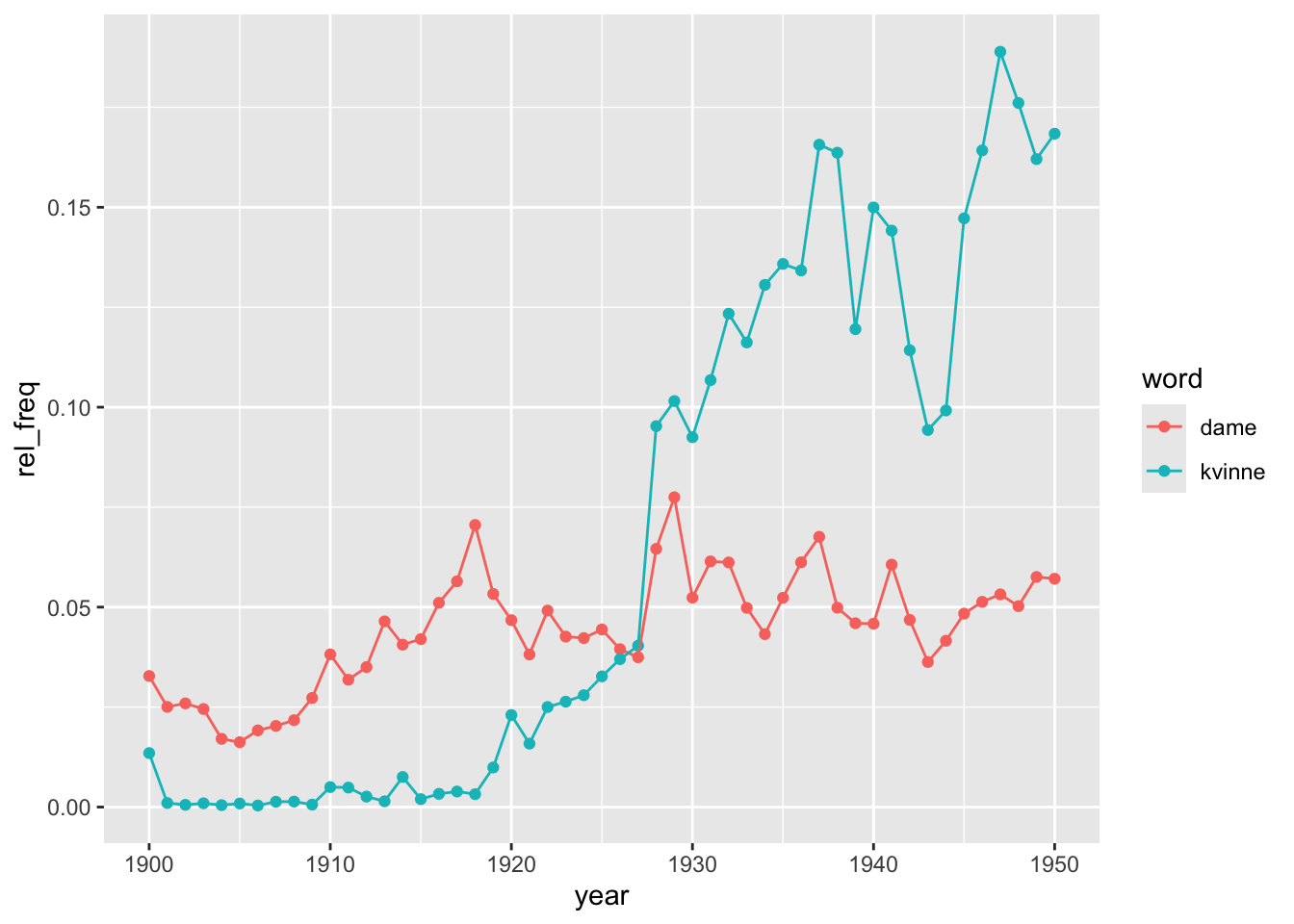

This analysis could be refined in many different ways. We could for instance explore what is behind these trends by distinguishing by genre or dropping the shortest or the longest texts to check whether the results are drive by a particular type of text. There could also be regional differences or by authorship, among other potential hypotheses. It is possible that the trends do not reflect real changes in language use but in the composition of the corpus. In general, always be careful with the composition of the sample in large-scale collections. Imagine that a bunch of specific records (e.g. periodicals, children lit, etc.), published between 1927 and 1940, make up for a significant fraction of the digitised texts present in the collection for that period. The use of “dame/r” and “kvinne/r” in those records would be driving the results but they might not be representative of the phenomenon we are studying.

Collocation

As well as getting term frequencies, the package dhlabR allows extracting the terms occurring next to the word we are interested in. The function get_collocations() works the same way as the one computing term frequencies. It requires providing a vector containing the unique identifiers of the texts in the corpus we are analysing (pid)), the target word (word) and the number of words before and after the target word to include as context (the default in 10 in both).

To limit computational requirements, let’s use a more limited corpus: the books published in the 1930s (a corpus with 10,698 items).

Show code

books <- get_document_corpus(
  doctype = "digibok", 
  from_year = 1930, to_year = 1939,
  lang = NULL,
  limit = 15000)

We now make the query for obtaining the words occurring next to “dame” within a window of 5 words (before and after). We can only query one term at a time but it is easy to append different data frames after if we wished so. The argument sample_size indicates the number of samples we are retrieving from the API (default is 5000). Instead of analyzing all occurrences of the word in the corpus, the function can analyze a random sample of them to reduce computations. Setting a higher number gets you closer to the full corpus but slows down the computations.

Show code

collocations <- get_collocations(
  pids = books$urn,
  word = "dame",
  before = 5,
  after = 5,
  sample_size = 10000)
collocations |> 
  head(n = 10)

             counts dist bdist
übønnhørlige      3    1   0.2
ell               8    2   0.2
Berger            3    1   0.2
misakte           3    1   0.2
flonel            2    1  0.25
sparess           2    1  0.25
Ørjan             2    1  0.25
Adelheid          2    1  0.25
Challenger        2    1  0.25
Bright            2    1  0.25

This function returns a data frame with three columns: counts, dist and bdist, as well as a list with the terms that are stored as row names (not as a column). counts is the number of times a particular term shows up within the specified window around the target word. dist and bdist are weighted distance score to identify how far from the target word (the latter is a bidirectional distance score). As before, the resulting data frame needs to be tuned before use (a bit involved to be sure because the resulting data frame may sometimes empty fields). For simplicity, let’s also drop the weighting fields:

Show code

collocations <- collocations |>  
  rownames_to_column("term") |>
  as_tibble() |>
  mutate(counts = map_int(counts, ~ if (length(.x) == 0) NA_integer_ 
                          else as.integer(.x[[1]])),
         dist   = map_dbl(dist,   ~ if (length(.x) == 0) NA_real_ 
                          else as.numeric(.x[[1]])),
         bdist  = map_dbl(bdist,  ~ if (length(.x) == 0) NA_real_ 
                          else as.numeric(.x[[1]]))) |>
  select(term, counts)
collocations

# A tibble: 20,669 × 2
   term         counts
   <chr>         <int>
 1 übønnhørlige      3
 2 ell               8
 3 Berger            3
 4 misakte           3
 5 flonel            2
 6 sparess           2
 7 Ørjan             2
 8 Adelheid          2
 9 Challenger        2
10 Bright            2
# ℹ 20,659 more rows

The most common terms next to “dame” are stop words (and punctuation symbols), as expected.

Show code

collocations |>
  arrange(desc(counts))

# A tibble: 20,669 × 2
   term  counts
   <chr>  <int>
 1 en     12236
 2 ,      10867
 3 .       9259
 4 og      4675
 5 som     4141
 6 med     3026
 7 var     2885
 8 i       2844
 9 den     2599
10 er      2022
# ℹ 20,659 more rows

We need to get rid of them. Extract Norwegian stop words. The function get_stopwords() from the tidytext package pulls stop words from different languages. Here we choose "no".

Show code

library(tidytext)
norsk_stop <- get_stopwords(language = "no")
norsk_stop

# A tibble: 176 × 2
   word  lexicon 
   <chr> <chr>   
 1 og    snowball
 2 i     snowball
 3 jeg   snowball
 4 det   snowball
 5 at    snowball
 6 en    snowball
 7 et    snowball
 8 den   snowball
 9 til   snowball
10 er    snowball
# ℹ 166 more rows

We then remove then from the previous object using anti_join() and present the most common terms occurring next to “dame”.

Show code

collocations |>
  anti_join(norsk_stop, by = c("term" = "word")) |>
  arrange(desc(counts))

# A tibble: 20,521 × 2
   term  counts
   <chr>  <int>
 1 ,      10867
 2 .       9259
 3 ung     1970
 4 »       1662
 5 «       1487
 6 En      1436
 7 —       1359
 8 unge    1183
 9 sig      948
10 ?        861
# ℹ 20,511 more rows

There are still some issues here. The most apparent is all those punctuation symbols but we can also see that upper- and lower-case letters might prevent identifying terms that are otherwise equal³ Although invisible, there might also be blanks at the beginning or at the end of a string that also count as characters and complicate identifying the same terms. The code below therefore removes potential blank spaces, converts all characters into lower-case and filters out rows containing symbols instead of letters using a regular expression that allows one or more of the specified characters between the start and the end of a string. Notice also that we are removing the stop words last because that list is all in lower-case characters, so doing it before transforming term into lower-case would miss many stop words whose first character appears capitalised.

³ Unless that we think that knowing that the term is at the beginning of a sentence is useful. Similarly, punctuation marks can also be informative. It all depends on what is our research question and which features of the corpus may help us better answer it.

Show code

collocations |>
  mutate(term = str_trim(term),
         term = str_to_lower(term)) |>
  filter(str_detect(term, "^[A-Za-zæøåÆØÅ]+$")) |>
  anti_join(norsk_stop, by = c("term" = "word")) |>  
  arrange(desc(counts))

# A tibble: 19,074 × 2
   term   counts
   <chr>   <int>
 1 ung      1970
 2 unge     1183
 3 sig       948
 4 gammel    727
 5 gamle     664
 6 sa        647
 7 mig       466
 8 liten     418
 9 ham       379
10 eldre     374
# ℹ 19,064 more rows

The results look much better and are very telling about the context in which the term dame is mentioned in this corpus.

Keywords in context

As well as counting the terms appearing next to the word we are interested in, we may want to have a look at the overall context in which those words appear. The function get_concordance() does the job for you. It works as the previous functions: it requires providing the text identifiers (pid), indicating the term (or terms) we are interested in (words) and specifying the window, the number of characters before and after the matching word that will be retrieved (default is 20). The optional argument limit indicates the maximum number of results to be returned (default is 5000). You will want all but here, which it is just an illustration, we set it to 20.

Show code

conc <- get_concordance(
  pid = books$urn,
  words = "dame",
  window = 30,
  limit = 20) 
conc |> glimpse()

Rows: 20
Columns: 3
$ docid <named list> 100571920, 100197025, 100373288, 100290192, 100234855, 10…
$ urn   <named list> "URN:NBN:no-nb_digibok_2007010500082", "URN:NBN:no-nb_dig…
$ conc  <named list> "... Var venn dlev glad , da det kom en <b>dame</b> inn o…

The function returns a data frame with two columns that identify the individual texts containing the target term and a column named conc with the text surrounding that keyword. As before, it needs a bit of tuning, so we have it in a more familiar format. You could now work on this data frame the same way you work with any other object we have been looking into.

Show code

conc |>
  as_tibble() |>
  mutate(docid = map_int(docid, 1),
         urn   = map_chr(urn, 1),
         conc  = map_chr(conc, 1)) |>
  select(docid, conc)

# A tibble: 20 × 2
       docid conc                                                               
       <int> <chr>                                                              
 1 100571920 "... Var venn dlev glad , da det kom en <b>dame</b> inn og avbrot …
 2 100197025 "... I vokslysets svake skjær så han en <b>dame</b> som ikke tilhø…
 3 100373288 "... Blandt disse var en <b>dame</b> fra Island , Sigridur Magnusd…
 4 100290192 "... Det var en ung , fin <b>Dame</b> — indsnøret og udsvaiet , me…
 5 100234855 "« Hvad er det egentlig for ærend De er ute i , unge <b>dame</b> ?…
 6 100067686 "... Jeg har ingen annen <b>dame</b> enn dig for øieblikket . Må j…
 7 100273203 "... Det var en vakker <b>dame</b> av ubestemmelig alder . Hun had…
 8 100465509 "gjøre den unge <b>dame</b> en slags erklæring , hvilken blev be *…
 9 100082744 "... En fortryllende <b>dame</b> sa at revolusjon er umulig , for …
10 100440097 "<b>Dame</b> med hatt . 1919. 32.5 x40 . Kunstneren ."             
11 100029451 "1 Wahl segjer svensk <b>dame</b> . Sjå hans bok « Johan Wibe » , …
12 100027313 "« <b>Dame</b> det ! Ei slik ei som går og brækjer i alt ! »"      
13 100176260 "lady ' Wdi <b>dame</b> ; l . ' s watch ( fl. ladies ' iratches ) …
14 100274644 "« Og her er Deres køie , unge <b>dame</b> , » sa han og pekte på …
15 100291050 "... Jeg forstår ikke . — Det er formodentlig ikke sedvanlig hos e…
16 100223103 "... De kom fint ut av det ingen sa noget om den annen kom hjem i …
17 100253201 "... Som nu den svenske skisserende <b>dame</b> og engelskmannen s…
18 100250866 "... Det var bare en eldre sykelig <b>dame</b> i huset sammen med …
19 100049455 "dagsvesper i 1886 da han uten tro og uten trang , av estetisk nyf…
20 100235862 "... 8 herrer , 1 <b>dame</b> . Scenen et sakførerkontor . 2. opla…

We finish here. The package dhlabR is still under development and scarcely documented. There are also other functions we have not explored such as get_dispersion(). If you are interested, you can find more details here.