2. In-class coursework: Numerical fields

This practice session is based on the summaries of the Spanish 1860 Population Census. This source reports information at the district level for the whole of Spain and is especially suited to study the educational levels of the population. As well as the name of each administrative unit (district) and the province it belonged to, the data set contains the number of males and females living in those districts who were illiterate (illit_m and illit_f), able to read (read_m and read_f) and able to write (write_m and write_f). You can find the data here (Beltrán Tapia and Martínez-Galarraga 2018) (the Canary Islands are not included).

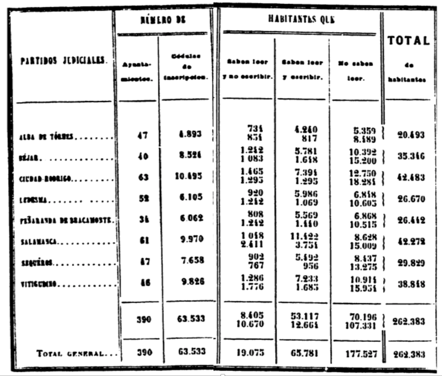
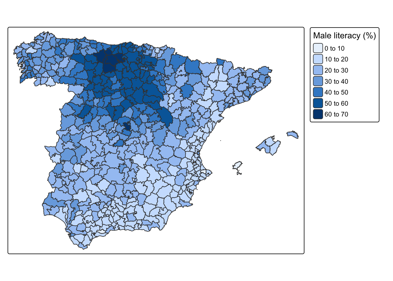
Sample image of the Statistical report based on the 1860 Spanish Census and male literacy rates by partido judicial (district). Source: INE Historia.

Male literacy rates by partido judicial (district), 1860.

Download the data set into a folder of your choice and read it into R. Remember to set the working directory and load the necessary packages. Note also that this is a .csv file, so you will need the function read_csv(), which is part of the tidyverse.
Explore how the data set looks like. How many observations does it contain? What each observations refers to (unit of analysis)? What kind of information does it report about each observation?
Compute literacy rates, that is, the percentage of the population who were able to read and write, for both males and females for each district. What are the minimum and maximum values of literacy? Identify the districts that perform best and worst in terms of literacy.
What is the average literacy rate?
Construct a histogram showing the full distribution of both male and female literacy rates.
Compute average male literacy rates at the province level. Do the same but weighting this measure by the existing male population. Which province ranked highest and lowest in terms of male literacy.

Solution

In my case, I downloaded the associated file, dist-1860.csv, in the folder data-assing, so after setting the working directory in the course folder, the code below imports it into the R environment. As mentioned above, the raw data is in a .csv file, so we use read_csv() to read it into R. Note that this function is already loaded when you load the tidyverse, so no further packages are needed (at least for now).

Show code

rm(list=ls())
setwd("~/Library/CloudStorage/OneDrive-NTNU/course-websites/computational-history")
library(tidyverse)
data <- read_csv("data-assign/educ-1860/dist-1860.csv")

Let’s explore how the data set looks like.

Show code

data

# A tibble: 464 × 8
   district           province  illit_m read_m write_m illit_f read_f write_f
   <chr>              <chr>       <dbl>  <dbl>   <dbl>   <dbl>  <dbl>   <dbl>
 1 Aguilar            Córdoba      9614    264    2081   10593    412     957
 2 Alba de Tormes     Salamanca    5359    734    4240    8489    854     817
 3 Albacete           Albacete     9031    362    2881   11196    372    1130
 4 Albaida            Valencia    11562    390    2378   13202    624     580
 5 Albarracín         Teruel       6743    391    3837   11757    292     449
 6 Alberique          Valencia     6125    163    1158    6835    189     269
 7 Albocázer          Castellón    9729    254    1400   10843    137     129
 8 Alburquerque       Badajoz      7774    202    1820    8592    270     585
 9 Albuñol            Granada     11268    323    2454   13942    348     624
10 Alcalá de Guadaira Sevilla      9107    464    2060    9540    508     863
# ℹ 454 more rows

As indicated at the top of the R output, this data frame contains 464 rows and 8 columns. This means that we have 8 pieces of information about the 464 districts existing in Spain in 1860 (these districts are administrative units similar to counties). We therefore have 464 observations and the associated information about them in terms of the province they belong to and the number of males and females that are illiterate, able to read and able to both read and write.

Let’s now compute literacy rates, that is, the percentage of the population who were able to read and write, for both males and females for each district. The source itself gives us the number of individuals of each sex in each group. For instance, for males, we have illit_m, read_m and write_m. Summing up the three groups would give us the total male population. We can therefore rely on this information to compute literacy rates. We can create new columns using mutate() and indicate how to calculate them. We do it below first for males and then for female:

Show code

data <- data |> 
  mutate(pop_m = illit_m+read_m+write_m,
         lit_m = 100*write_m/pop_m,
         pop_f = illit_f+read_f+write_f,
         lit_f = 100*write_f/pop_f)

Running the previous command does not yield any results because we are using the symbol <- to modify the existing object data. You could now use view(data) and scroll to the right to see the new columns that we have created. Alternatively, we are asking R to show one of them to us (lit_m), as well as the variables we use to calculation (at least the first 10 cases).

Show code

data |> 
  select(district, illit_m, read_m, write_m, pop_m, lit_m)

# A tibble: 464 × 6
   district           illit_m read_m write_m pop_m lit_m
   <chr>                <dbl>  <dbl>   <dbl> <dbl> <dbl>
 1 Aguilar               9614    264    2081 11959  17.4
 2 Alba de Tormes        5359    734    4240 10333  41.0
 3 Albacete              9031    362    2881 12274  23.5
 4 Albaida              11562    390    2378 14330  16.6
 5 Albarracín            6743    391    3837 10971  35.0
 6 Alberique             6125    163    1158  7446  15.6
 7 Albocázer             9729    254    1400 11383  12.3
 8 Alburquerque          7774    202    1820  9796  18.6
 9 Albuñol              11268    323    2454 14045  17.5
10 Alcalá de Guadaira    9107    464    2060 11631  17.7
# ℹ 454 more rows

We now know what the literacy rate in each district was. What about the average literacy? And the minimum and maximum values? As you will have probably guessed, we will need the functions summarize() plus the particular one depending on what we want to compute: sum(), mean(), sd(), min(), max(), etc. Let’s start with the minimum and maximum values

Show code

data |> 
  summarize(min = min(lit_m, na.rm = TRUE),
            max = max(lit_m, na.rm = TRUE))

# A tibble: 1 × 2
    min   max
  <dbl> <dbl>
1  8.01  64.0

The minimum and the maximum values indicate that there are two districts performing specially bad and especially well in terms of literacy: while in one, only 8 per cent of males are able to read and write, in another one more than 64 per cent of them are literate. You could easily identify the name of these districts by using filter().¹

¹ Alternatively, you could use arrange() and sort in ascending or descending order in terms of lit_m.

Show code

data |>
  filter(lit_m<8.1)

# A tibble: 2 × 12
  district province illit_m read_m write_m illit_f read_f write_f pop_m lit_m
  <chr>    <chr>      <dbl>  <dbl>   <dbl>   <dbl>  <dbl>   <dbl> <dbl> <dbl>
1 Coín     Málaga     11208    211     994   11998    319     523 12413  8.01
2 Pego     Alicante    7873    308     721    8314    213     151  8902  8.10
# ℹ 2 more variables: pop_f <dbl>, lit_f <dbl>

Show code

data |>
  filter(lit_m>64)

# A tibble: 1 × 12
  district province illit_m read_m write_m illit_f read_f write_f pop_m lit_m
  <chr>    <chr>      <dbl>  <dbl>   <dbl>   <dbl>  <dbl>   <dbl> <dbl> <dbl>
1 Riaño    León        2530    677    5710    7519   2021    1014  8917  64.0
# ℹ 2 more variables: pop_f <dbl>, lit_f <dbl>

Let’s now compute the average literacy rate for all districts (464 in total). We are going to compute both the mean and the weighted mean. The first one considers all districts equally, so it adds up their literacy rates and divides that value for the number of observations. This yiels an average literacy of 30.3 per cent. The second one weights each observation according to another dimension. Here we are using population, meaning that the literacy rate of larger districts will weight more when making the computations.² The weighted mean is now 31.3, a bit higher than before. This is because bigger districts (i.e. Madrid, Barcelona, etc.) tend to have higher literacy rates, so given them a bit more weight implies obtaining a slightly higher mean literacy.

² Note that the function weighted.mean() requires two arguments. The first one, lit_m, is the field we want to compute the average from. The second one, pop_m, defines the weights: here the size of each district in terms of the number of males.

Show code

data |> 
  summarize(mean = mean(lit_m, na.rm = TRUE),
            w_mean = weighted.mean(lit_m, pop_m, na.rm = TRUE))

# A tibble: 1 × 2
   mean w_mean
  <dbl>  <dbl>
1  30.3   31.3

We now have a sense of the average literacy, as well as the minimum and the maximum values. Let’s construct a histogram to see the full distribution of values. We are going to do it for both male and female literacy rates and then put the two histograms together using the package patchwork (you have to install it first if you haven’t done so before). Given that the range of values that the two variables (lit_m and lit_f) cover is quite different (female literacy is significantly lower everywhere), we are forcing the two graphs to show the same range of values in the x-axis, so the comparison is more homogenous.³

³ Drop that option if you want to see the difference.

Show code

hist_m <- data |>
  ggplot(aes(x = lit_m)) + 
  geom_histogram(binwidth = 1) +
  coord_cartesian(xlim = c(0, 70)) +
  scale_x_continuous("Male literacy (%)", breaks = seq(0, 70, 10))

hist_f <- data |>
  ggplot(aes(x = lit_f)) + 
  geom_histogram(binwidth = 1) +
  coord_cartesian(xlim = c(0, 70)) +
  scale_x_continuous("Female literacy (%)", breaks = seq(0, 70, 10))

# install.packages("patchwork")
library(patchwork)
hist_m + hist_f

Histograms depict how many observations (districts here) fall within different parts of the distribution of potential values.⁴ A significant number of districts exhibit low male literacy rates (<20-25 per cent). There are however many districts showing higher values and a non-negligible fraction have literacy rates over 50 per cent. By contrast, most districts have very low female literacy rates (<10 per cent). Only a few (three) have literacy rates over 30 per cent. These two plots help having a sense of what literacy rates looked like for males and females in mid-19^th-century Spain.

⁴ I chose binwidth = 1 but it is ok if you have chosen a different value and the bars are wider (not defining this option implies that R decides for you). Feel free to try other values and choose the plot that, in your judgement, is more informative without being too noisy (spiky).

⁵ We could have computed the weighted mean (by population) if we wanted to take into account that, within each province, some districts are bigger than others, so they are weighted more in the calculations.

Lastly, imagine that, instead of districts, you are interested in knowing what the province literacy rates are. Recall that one of the columns (province) in the data indicates to which province each district belongs to. This enables introducing a super useful command that we will employ quite often during the course: group_by(), which allows making computations separately within groups delimited by the categories included in this other variable. The code below groups district by province and then computes the average literacy for each group.⁵

Show code

data |>
  group_by(province) |>
  summarise(lit_m = mean(lit_m, na.rm = TRUE),
            lit_f = mean(lit_f, na.rm = TRUE))

# A tibble: 48 × 3
   province    lit_m lit_f
   <chr>       <dbl> <dbl>
 1 Albacete     20.2  6.24
 2 Alicante     15.2  5.13
 3 Almería      15.5  4.17
 4 Badajoz      22.2  8.60
 5 Baleares     18.4  5.88
 6 Barcelona    31.3  8.87
 7 Burgos       55.2 10.2 
 8 Castellón    16.2  3.36
 9 Ciudad Real  24.0  6.69
10 Coruña       30.0  4.71
# ℹ 38 more rows

Note that the resulting dataframe no longer have 464 rows (districts) but 48, which is the number of Spanish provinces (excluding the Canary Islands).

This is just one way of looking into the topics presented above. There are different ways of extracting information from the source. You need to find your own in the sense of feeling comfortable with what you are doing and confident about understanding what the different commands are doing and the results themselves. Feel free to play around with the code. For instance, you can remove options to see what they do.

References

Beltrán Tapia, Francisco J., and Julio Martínez-Galarraga. 2018. “Inequality and Education in Pre-Industrial Economies: Evidence from Spain.” Explorations in Economic History 69: 81–101.